Optimizing the Arduino Solar Tracker Build Pipeline
Building an arduino solar tracker is a staple microcontroller project, but transitioning from a jittery breadboard prototype to a reliable, field-deployable dual-axis system requires a disciplined engineering workflow. According to the National Renewable Energy Laboratory (NREL), dual-axis tracking can increase photovoltaic energy yield by up to 35% compared to fixed-tilt setups. However, this gain is entirely negated if the tracker suffers from parasitic power drain, mechanical stalling, or sensor noise. As of 2026, the maker ecosystem offers highly optimized components that, when assembled using a Design for Assembly (DFA) methodology, can reduce build time by 40% while eliminating the most common failure modes. This guide outlines a streamlined workflow for procurement, mechanical assembly, electrical isolation, and software calibration.
Phase 1: Strategic Component Procurement
The most common workflow bottleneck is under-specifying mechanical and electrical components, leading to mid-build redesigns. Standard SG90 micro servos strip their plastic gears within weeks of outdoor wind loading. Optimizing your Bill of Materials (BOM) upfront prevents costly iterations.
| Component | Recommended Model | Est. Cost | Workflow Rationale |
|---|---|---|---|
| MCU | Arduino Nano Every | $11.50 | ATmega4809 chip offers 10-bit ADC with improved sampling over legacy Nano; see official Arduino Nano Every docs. |
| Servos (x2) | TowerPro MG996R | $15.00 | Metal gears and 13kg-cm torque handle 12x12 inch panels without stalling. |
| Power Supply | LM2596 Buck Converter | $2.50 | Steps 12V solar battery down to 5.1V at 3A, isolating MCU from servo noise. |
| Light Sensors | GL5528 LDRs (x4) | $0.60 | High sensitivity (10-20kΩ at 10 lux) provides clean analog gradients. |
| Fasteners | M3 Brass Heat-Set Inserts | $4.00 | Prevents 3D-printed thread stripping during servo torque spikes. |
Phase 2: Mechanical Assembly & Tolerance Management
A chaotic mechanical assembly leads to binding, which spikes servo current draw and triggers software resets. To optimize the physical build workflow, adopt the following manufacturing standards:
Material Selection and 3D Printing Parameters
Do not use PLA for outdoor tracker housings; it undergoes glass transition at 60°C and will warp in direct sunlight. Print all structural brackets in PETG or ASA. For optimal rigidity without wasting print time, use a 40% gyroid infill with 3 perimeter walls. This specific slice profile balances print speed (under 4 hours for a full dual-axis gimbal) with the torsional rigidity needed to resist wind shear.
Eliminating Fastener Fatigue
Self-tapping screws into 3D-printed PLA or PETG will strip after three to four servo stall events. Integrate M3 brass heat-set inserts into your CAD models. Using a soldering iron set to 280°C, press the inserts into the printed holes. This creates a permanent metal-on-metal thread that survives infinite maintenance cycles, drastically reducing long-term maintenance workflow friction.
Pro-Tip: The Laser Pointer Calibration Jig
Aligning LDRs perfectly perpendicular to the panel is notoriously time-consuming. Tape a low-cost laser pointer to the center of your LDR cross-bracket. Project the beam onto a wall 10 feet away. This amplifies micro-degree misalignments, allowing you to file or adjust the bracket mounts to perfect zero-degree center in under 5 minutes, rather than relying on trial-and-error outdoor sun testing.
Phase 3: Electrical Isolation and Wiring Harnesses
Servo motors are inductive loads. When an MG996R changes direction or stalls, it injects severe Electromagnetic Interference (EMI) and voltage sags back into the power rail. If the MCU and servos share the same 5V rail without isolation, the Arduino will experience brownouts, corrupting its EEPROM and causing erratic tracking behavior.
Power Rail Segregation
- Main Input: Route your 12V solar battery input to a central terminal block.
- Servo Power: Connect the 12V input to the LM2596 buck converter. Adjust the potentiometer with a multimeter to output exactly 5.1V. Wire this directly to the servos' red and brown wires.
- MCU Power: Use a separate linear regulator (like an LM7805 with a heatsink) or feed the 12V into the Arduino Nano Every's VIN pin, letting its onboard regulator handle the logic power.
- Common Ground: Crucially, tie the ground of the buck converter and the MCU together at a single star-ground point to prevent ground loops.
Analog Signal Conditioning
LDRs output analog signals that are highly susceptible to noise from the servo PWM lines. To optimize signal integrity without adding complex op-amp circuits, use twisted-pair wiring for your LDR analog lines. Furthermore, solder a 100nF ceramic capacitor directly across the signal and ground pins of each LDR at the sensor end. This creates a hardware low-pass filter that smooths out high-frequency EMI, providing the MCU's ADC with a stable voltage to read.
Phase 4: Software Workflow & Hysteresis Calibration
The most critical software optimization in any arduino solar tracker is implementing hysteresis (a deadband). Without it, minor fluctuations in cloud cover or sensor noise will cause the tracker to 'hunt'—rapidly oscillating back and forth. This hunting behavior, as noted in Adafruit's motor selection guidelines, rapidly degrades servo potentiometers and wastes more power than the tracking gains provide.
Implementing the Deadband Algorithm
Instead of moving the servo every time the left LDR reads higher than the right LDR, introduce a threshold variable. Below is the logic flow for an optimized tracking loop:
- Read ADC values from Left, Right, Top, and Bottom LDRs.
- Calculate the horizontal error:
h_error = left_val - right_val. - Calculate the vertical error:
v_error = top_val - bottom_val. - The Optimization: Only actuate the horizontal servo if
abs(h_error) > 15. Only actuate the vertical servo ifabs(v_error) > 15. - Replace all
delay()functions with non-blockingmillis()timers to allow the MCU to handle serial logging or wind-sensor interrupts simultaneously.
Setting the deadband to ±15 ADC units (on a 10-bit scale of 0-1023) provides a physical tolerance of roughly 2 degrees of solar misalignment. Given that solar irradiance drops by less than 0.1% at a 2-degree offset, this trade-off saves massive amounts of mechanical wear and battery drain.
Phase 5: Troubleshooting Matrix & Field Deployment
Even with an optimized workflow, field conditions introduce variables. Use this diagnostic matrix to rapidly identify and resolve deployment issues without guessing.
| Symptom | Root Cause Analysis | Workflow Resolution |
|---|---|---|
| MCU resets when servos move | Voltage brownout due to servo stall current exceeding 2A. | Verify LM2596 output under load; upgrade to a 5A switching regulator if necessary. |
| Servos jitter continuously | Analog noise on LDR pins or missing software deadband. | Install 100nF caps on LDRs; increase software hysteresis threshold from 15 to 25. |
| Tracker drifts at night | LDRs reading ambient noise; lack of sleep mode. | Implement a 'Night Stow' routine that parks the panel flat when all 4 LDRs read below 50 ADC. |
| Gimbal binds at extreme angles | Wire harness tension or CAD clearance issues. | Use flexible silicone wire (22 AWG) and add cable chains to the azimuth axis. |
Weatherproofing for Longevity
To finalize the deployment workflow, house the MCU and buck converter in an IP65-rated ABS enclosure. Use PG7 cable glands for all wire exits to maintain the waterproof seal. Apply a conformal coating (such as MG Chemicals Silicone Modified) to the exposed solder joints on the LDRs to prevent humidity-induced corrosion, which alters their resistance curves over time.
Conclusion
By shifting your focus from ad-hoc prototyping to a structured, optimized workflow, you transform the arduino solar tracker from a weekend novelty into a robust, high-yield energy asset. Sourcing metal-gear servos, isolating power domains with buck converters, and enforcing strict software hysteresis are not just optional upgrades—they are mandatory engineering steps for any system intended to survive the realities of outdoor deployment. Implement these phases sequentially, and you will drastically reduce calibration time while maximizing your photovoltaic return on investment.