
The Anatomy of the Graph of Alternating Current
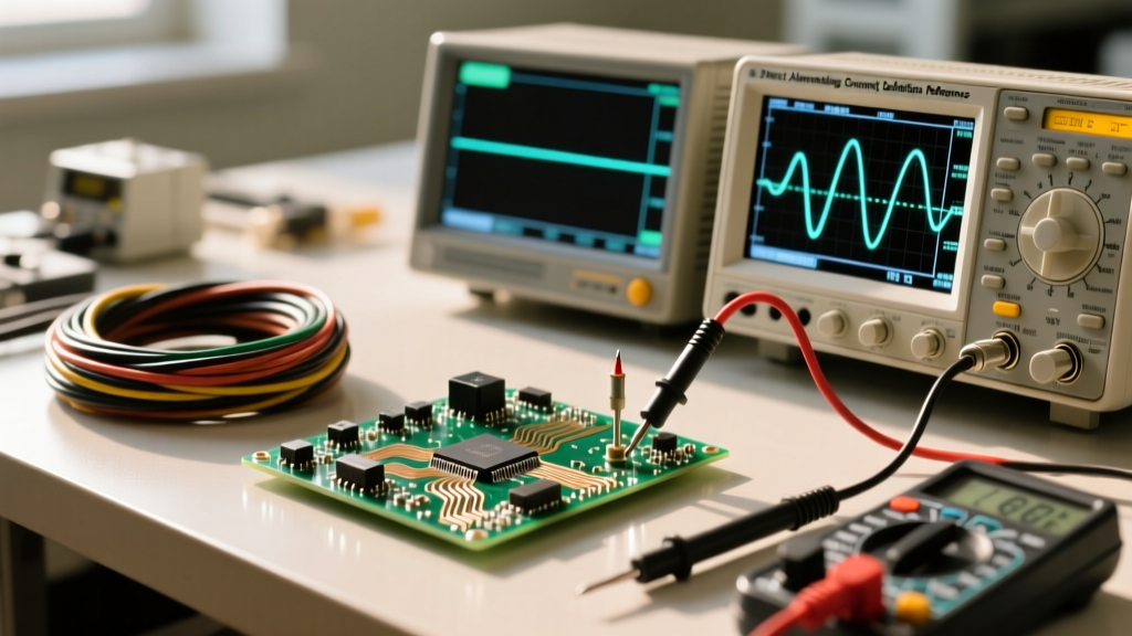
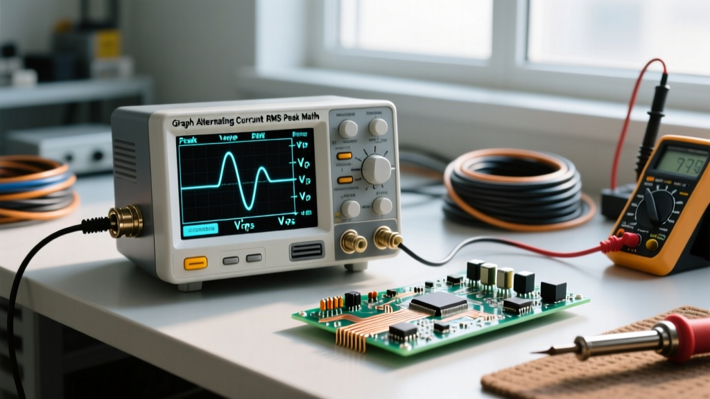
When you connect an oscilloscope to a live AC circuit, the resulting graph of alternating current reveals far more than a simple multimeter reading. While a standard digital multimeter averages out the waveform to provide a single Root Mean Square (RMS) value, the oscilloscope plots the instantaneous voltage and current over time. This visual representation—a sinusoidal wave—is the foundational blueprint for all AC electrical theory, wire sizing, and component selection.
Understanding this graph is not just an academic exercise; it is a critical skill for electrical DIYers and professionals. Misinterpreting the peak values on a graph of alternating current can lead to catastrophic insulation failure, while misunderstanding the RMS values can result in undersized conductors that overheat and cause fires. In this calculation tutorial, we will deconstruct the AC sine wave, master the core mathematical conversions, and apply these metrics directly to real-world wire sizing and circuit protection.
The Mathematical Framework of the Sine Wave
The standard graph of alternating current follows a trigonometric sine function. The instantaneous voltage v(t) at any given millisecond is calculated using the following formula:
v(t) = Vpeak × sin(2πft + θ)
- Vpeak: The maximum amplitude (the highest point on the Y-axis).
- f: Frequency in Hertz (Hz), representing cycles per second.
- t: Time in seconds (the X-axis).
- θ: Phase angle, representing a shift in the wave relative to a reference point.
For a standard North American 60Hz residential circuit, the wave completes 60 full cycles every second. Each cycle spans 360 degrees (or 2π radians), meaning the current crosses the zero-voltage axis 120 times per second. This continuous zero-crossing is precisely why AC arcs extinguish more easily than DC arcs, a vital factor when selecting circuit breakers and contactors.
RMS vs. Peak: The Insulation vs. Heating Paradox
The most common point of failure for beginners analyzing a graph of alternating current is confusing Peak voltage with RMS voltage. According to Fluke Corporation, True-RMS measurements are required for accurate power calculations, but peak values dictate dielectric stress.
RMS (Root Mean Square) is the effective heating value of the AC waveform. It is the equivalent DC voltage that would produce the exact same amount of heat in a resistive load. When the National Electrical Code (NEC) specifies ampacity tables for wire sizing, it is referencing RMS current. Thermal-magnetic circuit breakers also use RMS current to calculate thermal tripping curves.
Peak Voltage, however, is the absolute maximum electrical stress applied to wire insulation. The relationship between the two on a pure sine wave is:
VRMS = Vpeak × 0.7071 (or Vpeak / √2)
Vpeak = VRMS × 1.414
Real-World Application: THHN Insulation Limits
Consider a standard 480V RMS three-phase industrial system. A multimeter reads 480V. However, looking at the graph of alternating current, the peak voltage hitting the wire insulation is 480 × 1.414 = 678.7 Volts. Standard THHN wire insulation is rated for 600V RMS. While 600V RMS translates to an 848V Peak tolerance (safely covering the 678.7V peak), using a wire rated for only 300V RMS on this circuit would result in dielectric breakdown and arcing, even though the 'operating voltage' seems within a safe margin of error.
Data Table: Common AC System Waveform Metrics
The table below breaks down the critical values derived from the graph of alternating current for standard global power systems. These numbers dictate both conductor ampacity and insulation thickness.
| System Nominal (RMS) | Peak Voltage | Peak-to-Peak Voltage | Frequency | Period (ms) |
|---|---|---|---|---|
| 120V (US Residential) | 169.7 V | 339.4 V | 60 Hz | 16.67 ms |
| 240V (US Split-Phase) | 339.4 V | 678.8 V | 60 Hz | 16.67 ms |
| 230V (EU Standard) | 325.2 V | 650.4 V | 50 Hz | 20.00 ms |
| 480V (US Industrial) | 678.8 V | 1357.6 V | 60 Hz | 16.67 ms |
Time-Domain Calculations: Frequency and Phase Shift
The X-axis of the AC graph represents time. Calculating the period (T) of the wave is essential for troubleshooting power quality issues and sizing capacitors for power factor correction. The formula is simple:
T = 1 / f
In a 60Hz system, T = 1/60 = 0.01667 seconds, or 16.67 milliseconds per full cycle. If you are analyzing a multi-wire branch circuit (MWBC) using an oscilloscope, you might notice a phase shift between the current and voltage waveforms due to inductive loads like motors. This phase shift is measured in degrees or milliseconds. To convert a time delay (Δt) into a phase angle (θ), use the following calculation:
θ = (Δt / T) × 360°
For example, if the current waveform lags the voltage waveform by 4.16 milliseconds on a 60Hz grid (where T = 16.67ms), the phase angle is (4.16 / 16.67) × 360 = 89.8 degrees. This indicates a highly inductive load with a poor power factor, meaning the wire must be sized to handle the excessive reactive current that performs no real work but generates significant I²R heating.
Translating the Graph to Wire Sizing and Skin Effect
How does the visual frequency on the graph of alternating current impact physical wire sizing? The answer lies in the skin effect. As detailed by Georgia State University HyperPhysics, alternating current does not distribute evenly across the cross-section of a conductor. The changing magnetic field generated by the AC waveform forces electrons toward the outer 'skin' of the wire.
At standard 60Hz utility power, the skin effect is negligible for conductors smaller than 500 kcmil. However, in high-frequency applications (such as variable frequency drives, VFDs, or RF electronics), the frequency on the X-axis of our graph increases dramatically. At 10,000 Hz, the effective conductive area of a standard AWG 4 copper wire is drastically reduced, increasing AC resistance and causing severe overheating. To compensate, engineers must use Litz wire (multiple individually insulated strands) or tubular busbars to maximize surface area.
Step-by-Step Calculation Tutorial: Sizing a VFD Branch Circuit
Let us apply these concepts to a practical scenario. You are wiring a 10 HP, 240V three-phase motor controlled by a Variable Frequency Drive (VFD). The VFD uses Pulse Width Modulation (PWM), which drastically alters the standard graph of alternating current.
- Identify the RMS Current: The motor nameplate lists a Full Load Amps (FLA) of 28A RMS. Per NEC Article 430, you must size the conductors at 125% of FLA. 28A × 1.25 = 35A.
- Select Base Wire Size: According to NEC Table 310.16, an 8 AWG THHN copper wire rated at 90°C handles 55A, which is more than sufficient for the 35A RMS thermal requirement.
- Analyze the Peak Voltage and dV/dt: The VFD outputs high-frequency PWM pulses. The graph of alternating current here is not a smooth sine wave, but a series of square-ish pulses with extreme voltage spikes (due to cable capacitance and inductance). The peak voltage can reach 2 × 240V = 480V, and the rate of rise (dV/dt) can cause corona discharge.
- Adjust for Dielectric Stress: Standard THHN insulation may degrade prematurely under these high-frequency peak spikes. You must upgrade to specialized VFD-rated cable (often rated 2000V Peak) or use XHHW-2 insulation, which has a thicker dielectric barrier to withstand the harsh PWM waveform.
Expert Troubleshooting Tip: Never rely solely on a standard averaging multimeter when diagnosing non-linear loads like LED drivers or VFDs. The graph of alternating current for these devices is heavily distorted (rich in harmonics). You must use a True-RMS meter or a power quality analyzer to capture the actual heating value, otherwise, your wire sizing calculations will be dangerously optimistic.
Summary of AC Waveform Fundamentals
Mastering the graph of alternating current bridges the gap between abstract electrical theory and safe, code-compliant physical installations. By remembering that RMS dictates thermal wire sizing and breaker thresholds, while Peak voltage dictates insulation integrity and dielectric stress, you can design circuits that are both efficient and resilient. Always verify your time-domain metrics and account for harmonic distortion when dealing with modern solid-state electronics.
For further reading on AC waveform theory and complex impedance calculations, consult the comprehensive guides available at All About Circuits.