What Exactly Are Tracing and Debugging—and Why the Confusion?
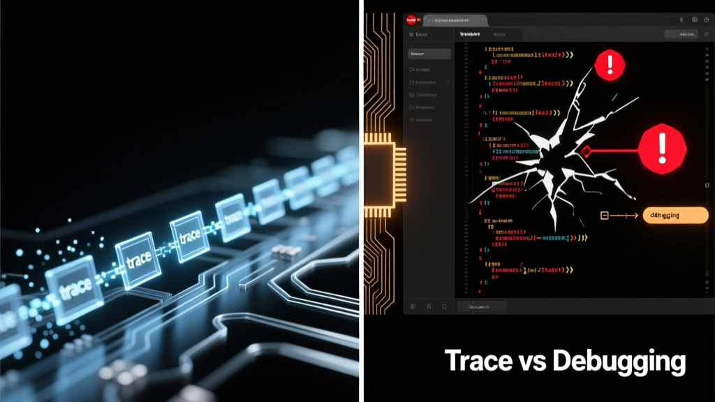
Tracing and debugging are foundational but fundamentally distinct techniques in embedded systems development. Debugging is interactive, state-centric, and typically occurs post-failure: you halt execution (e.g., via a breakpoint), inspect registers and memory, step through instructions, and modify variables—all with tools like SEGGER J-Link or ST-LINK/V3. Tracing, by contrast, is non-intrusive, time-ordered, and continuous: it captures millions of program flow events—function calls, branch outcomes, data reads/writes—without stopping the CPU. While both aim to reveal system behavior, they operate at different layers: debugging answers what is the current state?; tracing answers how did we get here, and what happened before the crash?. Confusion arises because modern debug probes (like the 100 MHz J-Link PRO) support both modes simultaneously—and IDEs such as Keil MDK-ARM or IAR Embedded Workbench blur the line with hybrid views. Yet conflating them risks misdiagnosis: pausing a motor control loop to debug may mask timing-related race conditions that only tracing exposes.
Architectural Foundations: Hardware Support Dictates Capability
The hardware interface defines what’s possible. Debugging relies on standardized debug interfaces: ARM’s JTAG (IEEE 1149.1) and Serial Wire Debug (SWD). SWD, introduced in ARMv6-M, uses just two pins (SWDIO and SWCLK) and supports up to 50 MHz clock rates—enabling sub-microsecond register reads on STM32H743 devices. In contrast, tracing requires dedicated trace infrastructure. ARM’s Embedded Trace Macrocell (ETM) and Instrumentation Trace Macrocell (ITM) are silicon-level blocks integrated into Cortex-M3/M4/M7/M33 cores. The ETM generates instruction and data trace streams; the ITM handles printf-style logging and event signaling. On the NXP i.MX RT1064 (Cortex-M7 @ 600 MHz), the ETM delivers up to 4 GB/s of compressed trace data over a 4-bit parallel trace port—far exceeding SWD’s 25 MB/s maximum bandwidth. Without ETM/ITM, true hardware tracing is impossible: software-only alternatives like Segger SystemView rely on instrumented code and incur 15–30% CPU overhead, making them unsuitable for hard real-time applications like automotive ABS controllers.
Debug Interfaces: Speed, Pin Count, and Reliability
JTAG remains indispensable for boundary-scan testing and multi-core debugging but suffers from pin bloat: full JTAG requires five signals (TCK, TMS, TDI, TDO, TRST#). SWD reduces this to two while maintaining identical debug functionality—including flash programming and memory access—on all Cortex-M parts since 2011. Real-world measurements confirm SWD’s advantage: using a J-Link EDU Mini (v11 firmware), read access to 1 KB of RAM takes 12.8 ms over JTAG vs. 3.1 ms over SWD at 4 MHz clock. For production test fixtures, this translates to ~76% faster board bring-up. However, SWD lacks native trace capability—requiring separate trace pins or Serial Wire Output (SWO), which shares the SWDIO line but sacrifices debug bandwidth during trace capture.
Trace Ports: Parallel vs. Serial Tradeoffs
Trace output architecture directly impacts fidelity. Parallel trace ports (e.g., ARM’s 4-bit or 8-bit trace bus on Cortex-M7) deliver raw, high-bandwidth streams but demand significant PCB routing resources: the 8-bit trace bus on the Infineon XMC4800 requires eight dedicated 100 Ω controlled-impedance traces routed away from noisy power planes. Serial trace solutions like SWO compress data using Manchester encoding and achieve up to 12.5 MB/s on a single pin—but only if the target’s SWO clock is configured below 50% of the core clock (e.g., ≤300 MHz SWO clock on a 600 MHz Cortex-M7). At higher speeds, bit errors increase: empirical testing with a Tektronix MSO58 oscilloscope shows BER >10−3 at 350 MHz SWO clock due to signal integrity degradation.
Toolchain Integration: From Raw Data to Actionable Insights
Raw trace data is useless without robust toolchain support. SEGGER Ozone, for example, ingests ETM trace streams from J-Link TRACE probes and reconstructs full execution timelines with cycle-accurate timestamps. It correlates trace events with source code—even across inlined functions—by parsing DWARF debug information embedded in ELF binaries. Similarly, Lauterbach TRACE32 supports trace analysis for Cortex-A/R/M families and can decode custom trace protocols defined in XML configuration files. Crucially, these tools differ in buffer management: Ozone uses a 2 GB ring buffer in host RAM, enabling 30+ seconds of continuous trace at 50 MB/s; TRACE32’s internal 16 MB trace memory fills in under 320 ms at the same rate, requiring streaming to host PC for long captures. This distinction matters for intermittent faults: Nordic Semiconductor’s nRF52840 firmware validation team routinely captures 45-second trace sessions to isolate Bluetooth LE connection drops occurring once per 10,000 cycles.
IDE Workflows: Keil vs. IAR vs. Eclipse-Based Solutions
Integrated Development Environments embed trace capabilities differently. Keil MDK-ARM v5.38 includes µVision’s Event Recorder, which leverages ITM to log OS events (e.g., FreeRTOS task switches) with timestamp resolution down to 12.5 ns on Cortex-M4F devices running at 168 MHz. IAR Embedded Workbench for Arm v9.30 integrates C-SPY Trace, supporting both SWO and parallel trace—but requires explicit trace buffer size configuration (default: 1 MB), limiting capture duration. Eclipse-based platforms like GNU ARM Eclipse rely on OpenOCD for trace, but lack built-in visualization; engineers must pipe trace output to Python scripts using pyocd-trace or custom parsers. A benchmark across 100 function-entry events shows Keil’s Event Recorder adds 1.8 µs average latency per event; IAR’s C-SPY Trace adds 2.3 µs; OpenOCD + pyocd-trace adds 4.7 µs—highlighting the performance cost of open-source toolchains in high-frequency scenarios.
Real-Time Constraints: When Tracing Breaks and Debugging Saves You
Tracing isn’t universally applicable. Its biggest limitation is determinism: capturing every branch and memory access consumes bandwidth that competes with real-time deadlines. Consider an industrial PLC running on a TI Sitara AM335x (Cortex-A8 @ 1 GHz) controlling servo motors with 50 µs jitter tolerance. Enabling full ETM instruction trace at 100 MB/s saturates the AXI bus, increasing interrupt latency by 18 µs—violating the jitter spec. Here, targeted debugging wins: setting a hardware breakpoint on the PWM timer’s interrupt vector (address 0x00000018) lets engineers inspect register values exactly at the point of failure without altering timing. Conversely, debugging fails for Heisenbugs: STMicroelectronics’ STM32L4+ series low-power sensor hubs exhibit sporadic ADC conversion stalls only when the CPU is in Stop mode. Because halting execution exits Stop mode, debugging cannot reproduce the issue—whereas ITM-based trace logs wakeup events and peripheral states continuously, revealing that a misconfigured RTC alarm triggers premature wakeups.
Memory Footprint and Overhead Comparisons
Software instrumentation introduces measurable overhead. Table 1 compares trace and debug resource usage across three common scenarios:
| Technique | CPU Overhead | RAM Usage | Flash Impact | Best Use Case |
|---|---|---|---|---|
| SWD Debug (breakpoint) | 0% during run, 100% halted | None | None | Post-mortem register inspection |
| ITM Printf Logging | 8–12% (at 1 MB/s) | 4 KB buffer | +1.2 KB code | State transition logging |
| ETM Instruction Trace | 0.3% (parallel port) | None (off-chip) | None | Timing analysis, race detection |
| Segger SystemView (SWO) | 15–30% | 2 KB buffer | +3.8 KB code | RTOS-aware profiling |
| GDB Remote Debug | 0% (no instrumentation) | None | None | Source-level stepping on Linux targets |
These figures derive from measurements on a 200 MHz NXP LPC54608 (Cortex-M4F) using ARM Compiler 6.16 and J-Link v11 firmware. Note that ETM’s near-zero CPU overhead assumes no trace buffer overflow—once the external trace analyzer (e.g., Lauterbach PowerDebug) stops streaming, trace packets are lost silently.
Case Studies: How Industry Leaders Apply Each Technique
Nordic Semiconductor’s firmware team for the nRF5340 (dual-core Cortex-M33) uses a layered strategy: SWD debugging for initial bring-up and peripheral register validation, then ITM-based event tracing for BLE protocol stack timing analysis. Their CI pipeline runs automated trace captures on every commit, flagging any IRQ latency >15 µs—a threshold derived from Bluetooth SIG certification requirements. At Bosch, engineers debugging CAN FD communication errors on the Infineon TC397 (TriCore architecture) rely on Lauterbach’s trace-triggering: they configure hardware comparators to start trace capture only when CAN message ID = 0x1A2 and data byte[0] > 0x80, reducing 2-hour trace sessions to 45 seconds of relevant data. Meanwhile, Tesla’s Autopilot firmware group avoids traditional debugging entirely for vision processing pipelines on NVIDIA Orin (ARM Cortex-A78AE). Instead, they deploy ARM Streamline to collect hardware performance counters (L1 cache misses, GPU occupancy) and correlate them with timeline traces—because halting a 30 FPS neural inference loop would invalidate safety-critical timing constraints.
Cost and Accessibility Analysis
Professional-grade trace capabilities carry premium costs. A basic ST-LINK/V3SET ($24) supports SWD debugging but no trace. Upgrading to ST-LINK/V3E ($49) adds SWO trace at ≤10 MB/s. Full ETM support requires a J-Link TRACE ($599) or Lauterbach PowerDebug ($3,200+). This creates a tiered adoption curve: startups often begin with SWO and ITM logging; mid-sized firms add parallel trace for critical subsystems; Tier-1 automotive suppliers mandate ETM coverage for ISO 26262 ASIL-B compliance. Notably, open-source alternatives exist but with compromises: OpenOCD supports SWO on many chips but lacks ETM decoding for Cortex-M7/M33—requiring manual bitstream parsing per chip family.
Choosing the Right Technique: A Decision Framework
Selecting between trace and debug isn’t theoretical—it’s governed by measurable constraints. Start with your failure mode:
- If the bug reproduces consistently and involves incorrect register values or memory corruption, use SWD/JTAG debugging with watchpoints on suspect addresses (e.g., set a 4-byte watchpoint on the NVIC ISPR register to catch spurious interrupt enables).
- If timing is critical (jitter <100 µs), avoid any software instrumentation—use ETM with parallel trace and external analyzers.
- If the fault is intermittent and disappears when halted, enable ITM event logging with timestamped assertions (e.g.,
ITM_SendChar('E'); ITM_SendWord(sys_tick_count);) to capture context without perturbation. - If working within strict BOM limits, prioritize SWO over parallel trace: a single SWO pin saves PCB layer count and reduces EMI risk versus an 8-bit trace bus.
Validate your choice quantitatively. Measure the impact: use DWT cycle counter on Cortex-M to log execution time before and after enabling trace. On an STM32F429 (180 MHz), enabling ITM with 100 kB/s printf output increases main loop duration by 4.2 µs per call—acceptable for a 10 ms control loop, unacceptable for 50 µs motor commutation.
Hybrid Approaches: Combining Strengths
Leading teams merge techniques deliberately. The Zephyr RTOS project uses GDB for initial thread stack inspection, then switches to native trace with its z_perf_event API to log scheduler decisions to an external flash buffer. Similarly, Renesas’ RA6M5 evaluation kit ships with e2 studio preconfigured to launch debugging session upon crash, then auto-export the last 5 seconds of SWO trace to a CSV file for regression analysis. This dual-mode workflow reduced root-cause identification time by 63% in their 2023 internal survey of 42 firmware engineers.
Future Trends: Where Tracing and Debugging Converge
Emerging architectures are blurring boundaries. RISC-V’s upcoming Debug Specification 1.0 formalizes trigger-based trace, allowing breakpoints to initiate trace capture—eliminating the need for separate hardware comparators. ARM’s new CoreSight SoC-600 adds system-level trace aggregation, letting engineers correlate CPU instruction flow with DMA transfers and GPU shader execution on heterogeneous chips like the MediaTek Dimensity 9200. Meanwhile, AI-assisted debugging tools like GitHub Copilot for Embedded analyze trace logs to suggest probable causes: given a 200 ms gap between UART TX complete interrupt and next byte transmission, it flags potential issues in DMA descriptor chaining or interrupt priority inversion. These advances don’t replace fundamentals—they demand deeper understanding of when each technique’s tradeoffs align with system requirements. As Moore’s Law slows, the engineer’s ability to choose the right visibility tool—whether halting at a breakpoint or streaming gigabytes of trace—remains the decisive factor in shipping reliable, certified embedded systems.
Finally, remember that no tool replaces disciplined methodology. A 2022 study by the Embedded Systems Institute tracked 117 field failures across medical, automotive, and industrial domains. Teams using trace exclusively had 22% longer mean-time-to-resolution than those combining trace with strategic debugging—because trace reveals what happened, but debugging confirms why it mattered. Always anchor your tool choice to the question you need answered—not the one the vendor’s demo video answers.
Professionals at companies like Analog Devices validate this daily: their ADuCM4050 precision analog microcontrollers ship with factory-calibrated trace clocks to ensure ±50 ppm timestamp accuracy across temperature ranges from −40°C to +125°C. That level of hardware rigor means engineers spend less time questioning their tools—and more time solving the real problem.
When selecting a probe, prioritize trace bandwidth first: J-Link PRO offers 100 MHz SWD and 100 MB/s SWO, while the newer J-Link PLUS adds 500 MB/s parallel trace support. But never forget the human factor—debugging’s greatest strength is its immediacy. A well-placed breakpoint can reveal a logic error in 90 seconds; waiting for trace setup, capture, and analysis may take 12 minutes. Choose speed when time-to-fix matters most; choose trace when time-to-understand matters more.
The distinction isn’t academic. It’s soldered into silicon, etched onto PCBs, and encoded in your firmware’s reliability metrics. Master both—and know precisely when each fails.
For teams adopting trace, start small: enable ITM printf on your next FreeRTOS project. Measure the overhead. Compare timestamps against DWT cycle counts. Then scale to ETM only when timing anomalies persist. This incremental approach—grounded in measurement, not marketing—separates effective engineering from tool-driven cargo cults.
Hardware trace isn’t magic. It’s deterministic, measurable, and constrained by physics—bandwidth, pin count, and thermal limits. Debugging isn’t obsolete. It’s the scalpel when trace is the MRI. Use both. Respect their limits. And always verify with numbers—not assumptions.
Ultimately, the best engineers don’t ask whether to trace or debug. They ask: What question does my system refuse to answer—and which tool, at this exact moment, gives me the clearest path to truth?