
The Physics of Deformation: Understanding the Strain Gauge
Interfacing a strain gauge with Arduino is a rite of passage for makers building digital scales, structural health monitors, or robotic force-feedback systems. However, a common beginner mistake is attempting to wire a raw strain gauge directly to an Arduino's analog input pins. To understand why this fails, we must first look at the physics of the piezoresistive effect.
A strain gauge is essentially a microscopic zig-zag pattern of conductive foil (often constantan or karma alloy) bonded to an insulating flexible backing. When the underlying material deforms, the foil stretches or compresses. This physical deformation changes the electrical resistance of the foil.
The Gauge Factor (GF): The sensitivity of a strain gauge is defined by its Gauge Factor. For standard metallic foil gauges, like the Vishay Micro-Measurements CEA series, the GF is typically around 2.0. This means a 1% change in length (strain) results in a 2% change in electrical resistance.
In real-world applications, the physical deformation is minuscule—often measured in microstrain (µε). For a standard 350Ω load cell experiencing 1000µε (a typical maximum for aluminum elastomers), the resistance change is a mere 0.07Ω. If you apply 5V across this gauge, the voltage change is in the microvolt range. The Arduino Uno's 10-bit ADC, referenced to 5V, has a resolution of roughly 4.88mV per step. It is physically impossible for the Arduino's native ADC to detect a microvolt shift. This is where bridge circuits and dedicated amplifiers become mandatory.
The Wheatstone Bridge: Translating Micro-Ohms to Millivolts
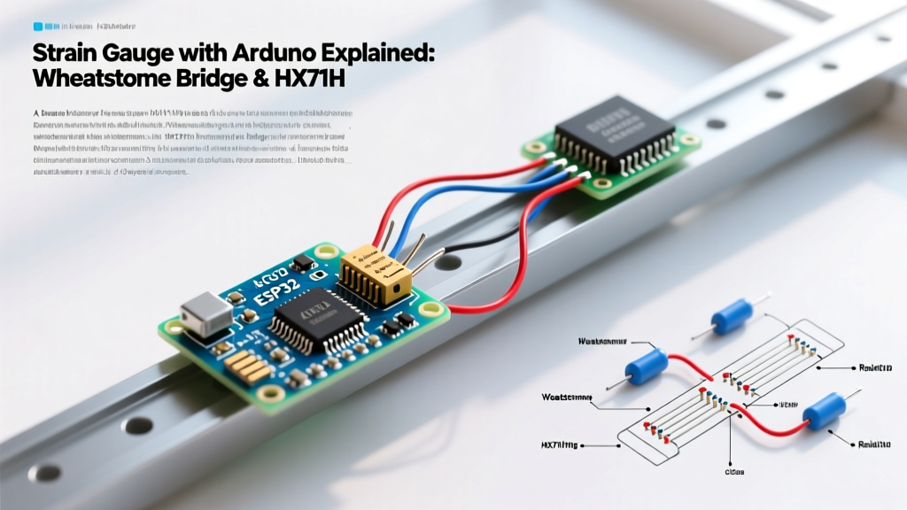
To measure these microscopic resistance changes, we arrange the strain gauge into a Wheatstone bridge circuit. This configuration uses four resistive arms to balance voltage. When the gauge deforms, the bridge becomes unbalanced, outputting a differential voltage proportional to the strain.
Most commercial load cells (like the TAL220 or CZL601) utilize a Full-Bridge configuration, integrating four active strain gauges. Two gauges experience tension while two experience compression, effectively multiplying the output signal by four compared to a single gauge, while simultaneously providing temperature compensation.
Bridge Configuration Comparison Matrix
| Configuration | Active Gauges | Output Sensitivity | Temperature Compensation | Typical Use Case |
|---|---|---|---|---|
| Quarter-Bridge | 1 | Low (Base) | Poor (Requires dummy gauge) | Experimental stress analysis |
| Half-Bridge | 2 | Medium (2x) | Good (If gauges are adjacent) | Bending beam measurements |
| Full-Bridge | 4 | High (4x) | Excellent (Inherent) | Commercial load cells, scales |
The HX711: Your 24-Bit Sigma-Delta Translator
Even with a full Wheatstone bridge, the maximum output is typically rated at 2mV/V. With a 5V excitation voltage, your maximum signal is only 10mV. You need massive amplification and high-resolution analog-to-digital conversion. Enter the HX711, a precision 24-bit analog-to-digital converter (ADC) designed specifically for weigh scales and industrial control applications.
As of 2026, the maker market is saturated with HX711 modules. While generic clones cost between $1.50 and $3.00, they often suffer from poor voltage references and noisy PCB layouts. For mission-critical projects, investing $12 to $18 in a breakout board from reputable vendors like SparkFun or Adafruit is highly recommended. These boards feature proper decoupling capacitors and stable LDO regulators for the analog excitation voltage.
Understanding HX711 Channels and Gains
The HX711 features two differential input channels, but they are not created equal:
- Channel A: Programmable gain of 128 (default) or 64. Used for the primary load cell signal.
- Channel B: Fixed gain of 32. Typically reserved for secondary sensors or temperature compensation thermistors.
Critical Timing Note: The HX711 does not use standard SPI or I2C. It uses a proprietary bit-bang serial protocol via two pins (DT and SCK). Furthermore, the datasheet specifies that keeping the SCK pin HIGH for more than 60µs puts the chip into power-down mode. Stray capacitance on long jumper wires can easily trigger this, causing the Arduino to read zeros. Keep your DT and SCK wires under 15cm, or use a localized pull-down resistor.
Step-by-Step Wiring Guide
Connecting a standard 4-wire load cell (such as a 10kg TAL220 half-bridge pair or a 50kg CZL601 full-bridge) to the Arduino via the HX711 requires careful attention to excitation and signal lines.
Load Cell to HX711 Pinout
- Red Wire (E+): Connect to HX711
E+(Excitation Positive) - Black Wire (E-): Connect to HX711
E-(Excitation Negative) - White Wire (A+): Connect to HX711
A-orA+(Signal Positive)* - Green Wire (A-): Connect to HX711
A+orA-(Signal Negative)*
*Note on Color Codes: While Red/Black/White/Green is the international standard, cheap direct-from-manufacturer load cells frequently swap the White and Green signal wires. If your scale reads negative values or erratic noise when weight is applied, simply swap the A+ and A- connections on the HX711 terminal block.
HX711 to Arduino Uno/Nano Pinout
- VCC: 5V (or 3.3V if using a 3.3V logic microcontroller like the ESP32)
- GND: Common Ground
- DT (Data): Digital Pin 2
- SCK (Clock): Digital Pin 3
Real-World Failure Modes and Edge Cases
Theoretical tutorials rarely prepare you for the noisy reality of embedded electronics. When deploying a strain gauge with Arduino in the field, you will encounter three primary failure modes.
1. Electromagnetic Interference (EMI) and 50/60Hz Mains Noise
Because the HX711 is amplifying microvolt signals, the wiring between the load cell and the amplifier acts as an antenna for AC mains hum. If your readings fluctuate by a few grams rhythmically, you are picking up 50Hz or 60Hz noise.
The Fix: Use twisted-pair shielded cable for the load cell wires, grounding the shield only at the HX711 end to prevent ground loops. Additionally, the HX711 has a RATE pin. Pulling this pin LOW sets the sample rate to 10 SPS (Samples Per Second), which inherently provides better rejection of 50/60Hz mains frequencies compared to the 80 SPS mode.
2. Thermal Drift and Apparent Strain
The resistance of the strain gauge foil changes with temperature, not just physical deformation. In a quarter-bridge setup, a 5°C room temperature shift can look identical to several kilograms of applied force. Full-bridge load cells mitigate this because all four gauges experience the same ambient temperature, causing their resistance shifts to cancel out mathematically within the bridge. Always use full-bridge load cells for environments lacking strict climate control.
3. Mechanical Creep and Hysteresis
If you leave a 20kg weight on a 50kg load cell for 24 hours, the Arduino will slowly report the weight dropping to 19.8kg. This is creep—the mechanical relaxation of the aluminum or steel elastomer. Conversely, when you remove the weight, the sensor might not return to absolute zero (hysteresis). Software cannot fix physical creep; you must implement an auto-tare routine in your code that triggers when the system detects a stable, unchanging baseline for a set duration.
Calibration Math: From Raw ADC to Kilograms
The HX711 library outputs a raw 24-bit signed integer, typically ranging from -8,388,608 to +8,388,607. To convert this to meaningful engineering units, you must perform a two-point calibration.
- Find the Offset (Tare): With zero load, read the raw value over 20 samples and average it. This is your
OFFSET. - Find the Scale Factor: Place a precisely known mass (e.g., a 10.000 kg calibration weight or a verified dumbbell) on the sensor. Read the new averaged raw value.
- Calculate:
SCALE = (Raw_Loaded - OFFSET) / Known_Weight_kg
In your main loop, the final weight is calculated as: Weight = (Raw_Reading - OFFSET) / SCALE. Implementing a simple moving average filter (averaging the last 10 to 15 readings) in software will smooth out the remaining high-frequency ADC jitter, yielding a stable, professional-grade measurement system.