
The Physics Baseline: Lorentz Force in 3D Space
In advanced electronics prototyping—specifically when designing vacuum tubes, cathode ray displays, mass spectrometers, or electron beam lithography systems—precise beam steering is critical. To steer an electron beam, engineers must accurately determine the x-component of the force on the electron as it traverses electromagnetic fields. This force is governed by the Lorentz force law, which in three-dimensional Cartesian coordinates defines the x-component as:
Fx = q(Ex + vyBz - vzBy)
Where q is the elementary charge of an electron (approximately -1.602 × 10⁻¹⁹ Coulombs, as defined by the NIST CODATA fundamental physical constants), E represents the electric field vector, v is the velocity vector, and B is the magnetic flux density vector. While the equation is straightforward, applying it to real-world physical prototypes introduces complex variables like fringe fields, space charge effects, and relativistic mass increases. Below, we compare three distinct methodologies to determine this force, ranging from rapid analytical approximations to high-fidelity simulations and physical empirical testing.
Alternative 1: Analytical Hand Calculations (The Uniform Field Approximation)
The most accessible way to determine the x-component of the force on the electron is through analytical hand calculations, assuming idealized, uniform fields. This approach is standard during the initial schematic phase of designing electrostatic deflection plates.
Execution and Parameters
Assume an electron traveling primarily along the z-axis (vz ≈ v, vx = vy = 0) entering a pair of parallel deflection plates oriented to create an electric field purely in the x-direction. If the magnetic field is zero (B = 0), the Lorentz equation collapses to:
Fx = qEx
If you apply a potential difference (V) of 500V across two aluminum deflection plates spaced 10 mm apart (d = 0.01 m), the uniform electric field is Ex = V/d = 50,000 V/m. The resulting x-component of the force is:
Fx = (-1.602 × 10⁻¹⁹ C) × (50,000 V/m) = -8.01 × 10⁻¹⁵ Newtons.
Limitations and Edge Cases
Analytical calculations completely fail to account for fringe fields at the edges of the deflection plates. In reality, the electric field bows outward at the plate boundaries, meaning Ex is not perfectly uniform. For short plates or high-precision applications (like electron microscopy), relying solely on analytical math will result in beam positioning errors exceeding 5-10%. Furthermore, this method assumes a vacuum and ignores the mutual repulsion of electrons (space charge) within the beam itself.
Alternative 2: Finite Element Method (FEM) Simulations
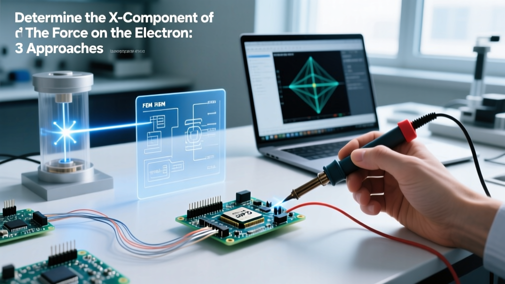
For modern vacuum electronic prototyping, numerical simulation is the industry standard. FEM software allows engineers to determine the x-component of the force on the electron by mapping the exact electromagnetic topology, including complex 3D geometries and fringe effects.
Software Ecosystem: FEMM vs. COMSOL
- FEMM 4.2 (Finite Element Method Magnetics): An open-source, Windows-based tool ideal for 2D planar and axisymmetric problems. According to the FEMM 4.2 Documentation, it excels at calculating electrostatic and magnetostatic fields. It is free but requires manual post-processing (via Lua scripting) to extract the exact force vector along a defined particle trajectory.
- COMSOL Multiphysics 6.2 (AC/DC & Particle Tracing Modules): A premium, fully 3D multiphysics environment. COMSOL automatically couples the electromagnetic field solver with relativistic particle tracking. Licensing costs typically exceed $10,000 annually, but it provides unparalleled accuracy for complex geometries like Einzel lenses and magnetic quadrupoles.
Simulation Setup Protocol
- Geometry & Materials: Define the vacuum chamber envelope and assign a relative permittivity (εr) of 1.0. Import the CAD model of your deflection yoke or plates.
- Boundary Conditions: Apply Dirichlet boundary conditions (fixed voltage) to the deflection electrodes. Apply Neumann (zero flux) or infinite element domains to the outer vacuum chamber walls to simulate open space.
- Mesh Refinement: This is the most critical step. You must apply a localized mesh refinement (element size ≤ 0.1 mm) in the gap between the deflection plates and along the expected electron trajectory. A coarse mesh will artificially smooth out the fringe fields, leading to an underestimation of Fx at the plate edges.
- Particle Tracing: Inject the electron with an initial kinetic energy (e.g., 10 keV). The solver calculates the local E and B fields at each time step, dynamically updating Fx as the electron's velocity vector changes.
Alternative 3: Empirical Measurement via Deflection Sensitivity
When simulation models lack precise material properties (e.g., unknown secondary emission yields or exact work functions of aged cathodes), empirical measurement becomes necessary. By building a physical test jig, you can determine the x-component of the force on the electron by measuring the physical displacement of the beam on a phosphor screen and back-calculating the force using kinematics.
Building the Test Jig
Construct a small-scale cathode ray tube using a commercial electron gun (such as the Kimball Physics EMG-12, which provides a stable, focused beam at variable acceleration voltages up to 10 kV). Mount your prototype deflection plates inside the vacuum envelope (maintained at < 10-6 Torr using a turbomolecular pump). Position a P43 (green-emitting, high-efficiency) phosphor screen at a known distance L from the center of the deflection plates.
Back-Calculating Fx
Apply a known voltage to the plates and measure the horizontal displacement (Δx) of the beam spot on the calibrated phosphor screen using a digital microscope. Using the kinematic equation for constant acceleration (valid only in the uniform region of the plates):
Δx = (Fx / me) * (l / vz) * [ (l / 2vz) + (L / vz) ]
Where me is the electron rest mass (9.109 × 10⁻³¹ kg), l is the physical length of the deflection plates, and vz is the axial velocity derived from the gun's acceleration voltage. By rearranging this formula, you can empirically solve for the average Fx experienced by the electron. This method inherently captures real-world anomalies like stray magnetic fields from the Earth or nearby lab equipment, which simulations often miss.
Comparison Matrix: Which Method Should You Choose?
| Methodology | Setup Time | Estimated Cost | Fringe Field Accuracy | Best Application Scenario |
|---|---|---|---|---|
| Analytical Calculation | < 10 Minutes | $0 (Free) | Poor (Ignores edges) | Initial proof-of-concept, basic classroom demonstrations, rough voltage estimations. |
| FEM Simulation (2D/3D) | 4 to 40 Hours | $0 (FEMM) to $10k+ (COMSOL) | Excellent (Highly precise) | Designing magnetic yokes, optimizing Einzel lenses, minimizing beam aberrations. |
| Empirical Measurement | 2 to 6 Weeks | $5,000 - $25,000 (Vacuum hardware) | Ground Truth (Captures all real-world variables) | Final prototype validation, calibrating mass spectrometers, troubleshooting unexpected beam drift. |
Edge Cases and Failure Modes in Prototyping
Regardless of the method you choose to determine the x-component of the force on the electron, advanced prototypers must account for non-ideal physics that can derail a design.
1. Space Charge Effects (Child-Langmuir Law)
If your electron gun operates at high current densities (e.g., > 1 mA/mm²), the mutual electrostatic repulsion of the electrons creates an internal electric field that opposes the external deflection field. This 'space charge' effectively shields the inner electrons from the full applied Ex, reducing the actual Fx compared to theoretical calculations. To mitigate this, FEM simulations must utilize self-consistent Poisson solvers rather than simple electrostatic approximations.
2. Relativistic Mass Corrections
The standard kinematic equations assume the electron mass is constant. However, if your acceleration voltage exceeds 10 kV, the electron's velocity approaches a significant fraction of the speed of light (c). At 50 kV, an electron travels at roughly 0.41c, and its relativistic mass increases by approximately 10%. If you fail to apply the Lorentz factor (γ) to the mass term in your empirical back-calculations, your derived Fx will be skewed. Modern solvers like the COMSOL AC/DC Module handle relativistic corrections automatically, but hand calculations require manual adjustment.
Expert Prototyping Tip: When using empirical measurement to find Fx, always perform a 'zero-field' baseline test. Even with deflection plates grounded, the electron beam may drift due to the Earth's magnetic field (approx. 25 to 65 μT depending on latitude) or residual magnetization in your vacuum chamber's stainless steel flanges. Subtract this baseline displacement from your powered measurements to isolate the true force generated by your prototype components.
Conclusion
Learning how to accurately determine the x-component of the force on the electron is a foundational skill for anyone working in vacuum electronics, particle physics, or advanced display prototyping. While analytical hand calculations provide a rapid starting point for uniform fields, they are insufficient for modern, high-precision devices. Integrating 2D or 3D FEM simulations allows for rigorous optimization of fringe fields and complex geometries. Finally, empirical measurement remains the ultimate arbiter of truth, capturing the messy, real-world variables that no software can perfectly predict. By strategically combining these three approaches, engineers can transition from theoretical physics to robust, functional hardware with confidence.