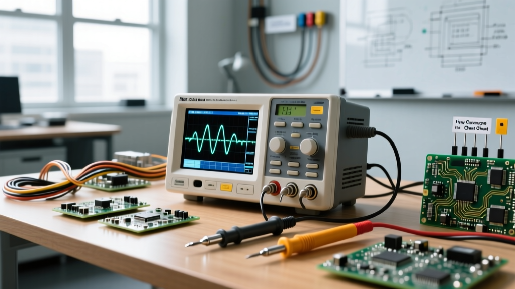
When technicians and engineering students ask, 'how does oscilloscope work?', the answer requires looking past the graphical display and into the complex analog-to-digital signal processing pipeline. Unlike a simple multimeter that provides a time-averaged scalar value, a Digital Storage Oscilloscope (DSO) captures voltage as a continuous function of time. This reference guide bypasses marketing fluff and provides a structural cheat sheet of the internal architectures, triggering logic, and sampling mathematics found in modern workhorses like the Rigol DS1054Z, Siglent SDS1202X-E, and Tektronix TBS1102B.
The Core Anatomy: Block Diagram Breakdown
To understand how an oscilloscope works, you must dissect its three primary hardware subsystems. According to Tektronix Oscilloscope Fundamentals, these systems operate in parallel but serve distinct signal-conditioning roles:
- Vertical System (Analog Front End): The signal enters through the BNC connector, passing through a TVS diode protection network. It then hits a stepped attenuator (e.g., 10:1 or 100:1) followed by a variable-gain pre-amplifier. This scales the input voltage to match the strict full-scale input range of the Analog-to-Digital Converter (ADC), typically ±500mV.
- Horizontal System (Timebase & Acquisition): This dictates the sampling clock. The ADC digitizes the scaled analog voltage at precise intervals (e.g., 1 GSa/s). The digitized words are then serialized and pushed into the acquisition memory (RAM), which dictates the maximum record length (e.g., 10 Mpts to 200 Mpts).
- Trigger System (Synchronization): A parallel analog comparator monitors the raw input signal against a user-defined voltage threshold. It generates a hardware logic 'START' pulse that aligns the acquisition memory buffer, ensuring repetitive waveforms appear stationary on the screen.
Signal Processing Pipeline: Step-by-Step Flow
Trace a 5V, 10 MHz square wave from the probe tip to the LCD pixels:
- Probe Attenuation: A 10X passive probe divides the 5V signal to 0.5V, while introducing a ~9 MΩ series resistance and a parallel compensation capacitor.
- Input Coupling: The user selects AC or DC coupling. DC passes the entire signal; AC engages a series high-pass filter capacitor to block DC offsets.
- Bandwidth Limiting: An optional 20 MHz low-pass filter can be engaged via relays to eliminate high-frequency switching noise from SMPS circuits.
- ADC Quantization: An 8-bit ADC maps the continuous voltage into 256 discrete digital levels (2^8). High-end models like the Siglent SDS2000X Plus use 10-bit ADCs (1024 levels) for finer vertical resolution.
- DSP Interpolation: Sin(x)/x digital interpolation algorithms connect the discrete sample points to render a smooth vector trace on the display grid.
Quick Reference: Triggering Modes Cheat Sheet
Misunderstanding trigger modes is the #1 reason beginners fail to capture elusive glitches. Electronics Notes outlines the foundational modes, but modern DSOs expand on these significantly:
| Trigger Mode | Behavior | Ideal Use Case |
|---|---|---|
| Auto | Forces a sweep if no trigger event occurs within a timeout period. | Initial setup; viewing unknown or drifting DC signals. |
| Normal | Screen freezes until the exact trigger condition is met. | Capturing low-duty-cycle PWM or intermittent serial packets. |
| Single | Arms once, captures the first valid trigger, then stops acquisition. | Debugging power-on reset sequences or capacitor inrush currents. |
| Runt | Triggers on pulses that cross one threshold but fail to cross a second. | Finding marginal logic levels or signal integrity violations on I2C. |
| Window | Triggers when a signal enters or exits a specific upper/lower voltage band. | Monitoring power supply ripple excursions outside of ±5% tolerance. |
Sampling Methods: Real-Time vs. Equivalent-Time
How does an oscilloscope work when measuring signals faster than its native ADC clock? It relies on Equivalent-Time Sampling (ETS).
Engineering Rule of Thumb: Real-Time Sampling (RTS) is mandatory for single-shot, non-repetitive events (like a microcontroller UART burst). ETS only works on perfectly periodic, repetitive signals by stitching together samples from multiple successive trigger cycles to build a high-resolution composite waveform.
If you attempt to use ETS on a single-shot I2C transaction, the oscilloscope will display aliasing artifacts or an entirely blank screen because the signal does not repeat to allow the timebase to interleave the samples.
Common Measurement Artifacts & Troubleshooting
Even when you understand how an oscilloscope works internally, external physics can corrupt your data. Watch for these specific failure modes:
1. Aliasing (The Nyquist Violation)
As defined by the Nyquist-Shannon Sampling Theorem, you must sample at least twice the highest frequency component of a signal. In practice, digital scopes require a 2.5x to 4x oversampling ratio for accurate Sin(x)/x reconstruction. If you measure a 100 MHz clock with a scope set to 100 MSa/s, the display will show a false low-frequency beat signal (aliasing). Fix: Always max out the sample rate and use the 'Peak Detect' acquisition mode to catch narrow glitches between sample intervals.
2. Ground Lead Inductance Ringing
The standard 6-inch alligator ground clip included with passive probes introduces approximately 10-15 nH of parasitic inductance per millimeter. When measuring fast-switching nodes (like a MOSFET drain or a buck converter switch node), this inductance forms an LC tank circuit with the probe's tip capacitance (~10 pF), causing massive high-frequency ringing that doesn't actually exist on the PCB. Fix: Remove the plastic probe hood and ground clip, and use a 'ground spring' or solder a bare wire directly to the probe tip barrel for sub-nanosecond edge fidelity.
3. Probe Compensation Mismatch
If the square wave on your scope's 1 kHz calibration terminal looks rounded (over-compensated) or exhibits overshoot spikes (under-compensated), the RC time constants of the probe and the scope's input impedance are mismatched. Use a non-metallic ceramic adjustment tool to tweak the trimmer capacitor on the probe compensation box until the edges are perfectly flat.
Bandwidth & Sample Rate Decision Matrix
Use this matrix to determine the required oscilloscope specifications based on the Device Under Test (DUT). Remember that for digital signals, the fundamental frequency is irrelevant; the rise time and harmonic content dictate the required bandwidth.
| Target Signal / Protocol | Typical Edge Rate | Required Scope Bandwidth (5x Rule) | Minimum Sample Rate |
|---|---|---|---|
| Audio / Analog Sensors | Slow (ms range) | 5 MHz | 25 MSa/s |
| UART / I2C (100 kHz) | ~1 µs | 20 MHz | 100 MSa/s |
| CAN Bus / RS-485 | ~10 ns | 100 MHz | 500 MSa/s |
| USB 2.0 Full Speed | ~4 ns | 500 MHz | 2.5 GSa/s |
| DDR3 Memory / PCIe | < 500 ps | 4 GHz+ | 20 GSa/s |
By internalizing this signal flow and referencing these hardware limitations, you transition from merely looking at squiggly lines to performing rigorous, quantitative time-domain analysis.