
Beyond the Textbook: The True Conductor Definition for Science
When students and DIYers first search for the conductor definition for science, they usually encounter a simplified physics textbook answer: a material that permits the free flow of electrical current due to loosely bound valence electrons. While this band-theory explanation is fundamentally correct, it is practically useless for electrical engineering, circuit design, and real-world wiring. In applied electrical science, a conductor is not just a material; it is a quantifiable, calculable pathway with specific resistive properties, thermal limits, and geometric constraints.
At Electrical Flux, we bridge the gap between theoretical physics and practical DIY electronics. To truly understand conductors, you must move beyond qualitative definitions and master the mathematics of resistivity, circular mils, and temperature coefficients. This calculation tutorial will equip you with the exact formulas used by electrical engineers to size wires, predict voltage drop, and prevent catastrophic thermal failures.
The Math Behind the Flow: Calculating Conductor Resistance
The fundamental property that defines a conductor's efficiency is its resistivity ($\rho$), measured in ohm-meters ($\Omega \cdot m$). However, in practical US-based electrical wiring, we rarely use meters. We use feet and Circular Mils (CM). To calculate the exact resistance ($R$) of a specific wire run, we use the adapted engineering formula:
$R = \frac{K \times L}{CM}$
Where:
R = Resistance in Ohms ($\Omega$)
K = Specific resistance of the material (Ohms-CM/ft)
L = Total length of the wire in feet (including the return path for DC/single-phase)
CM = Cross-sectional area in Circular Mils
A Circular Mil is the area of a circle with a diameter of one mil (1/1000th of an inch). The beauty of the CM system is that it eliminates $\pi$ from the calculation. To find the CM of any wire, you simply square its diameter in mils ($CM = d^2$). According to the Copper Development Association, the $K$ value for annealed copper at 20°C is approximately 10.4, while for aluminum, it is roughly 17.0.
Step-by-Step Calculation Example: 12 AWG Copper
Let us apply this to a real-world scenario. You are wiring a 20A, 120V receptacle circuit and need to run 50 feet of 12 AWG solid copper wire from the breaker panel to the outlet. What is the exact resistance and voltage drop?
- Step 1: Identify the CM. A standard 12 AWG wire has a diameter of 80.81 mils. Squaring this ($80.81^2$) gives us 6,530 CM.
- Step 2: Determine Total Length (L). For a complete circuit (hot and neutral), the current travels 50 feet out and 50 feet back. Total $L = 100$ feet.
- Step 3: Calculate Resistance. $R = \frac{10.4 \times 100}{6530} = 0.159 \Omega$.
- Step 4: Calculate Voltage Drop. Using Ohm's Law ($V = I \times R$), at a maximum continuous load of 16A (80% of a 20A breaker), the drop is $16 \times 0.159 = 2.54V$.
A 2.54V drop on a 120V circuit is a 2.1% voltage drop, which is well within the NEC recommended maximum of 3% for branch circuits.
Material Showdown: Conductivity vs. Resistivity Data Table
The conductor definition for science encompasses a wide spectrum of materials. While silver is the most conductive elemental metal, copper is the universal standard against which all other conductors are measured, known as the International Annealed Copper Standard (IACS). Below is a comparative data table of common conductive materials used in electrical and electronic applications.
| Material | Resistivity ($\Omega \cdot m$ at 20°C) | Conductivity (% IACS) | Specific Gravity | Primary DIY / Engineering Use Case |
|---|---|---|---|---|
| Silver (Ag) | $1.59 \times 10^{-8}$ | 105% | 10.49 | High-end audio contacts, RF shielding, aerospace |
| Copper (Cu) | $1.68 \times 10^{-8}$ | 100% (Baseline) | 8.96 | Standard branch wiring, PCB traces, magnet wire |
| Gold (Au) | $2.44 \times 10^{-8}$ | 70% | 19.30 | Corrosion-resistant edge connectors, IC bonding |
| Aluminum (Al) | $2.82 \times 10^{-8}$ | 61% | 2.70 | Service entrance cables, heavy feeder lines, transmission |
| Tungsten (W) | $5.60 \times 10^{-8}$ | 31% | 19.25 | Incandescent filaments, high-temp vacuum environments |
Temperature Coefficients: When Science Meets Real-World Heat
A critical flaw in basic science education is teaching resistivity as a static constant. In reality, as current flows through a conductor, $I^2R$ heating occurs. As the conductor's temperature rises, lattice vibrations (phonons) increase, causing more frequent electron scattering. This increases resistance. For precise engineering, you must calculate the hot resistance using the temperature coefficient formula:
$R_T = R_{20} [1 + \alpha (T - 20)]$
Where $\alpha$ is the temperature coefficient of resistance (for copper, $\alpha \approx 0.00393 / °C$). If our 12 AWG copper wire from the previous example reaches 75°C (the standard temperature rating for most modern breaker terminals and THHN insulation), the resistance changes significantly:
- $R_{75} = 0.159 \times [1 + 0.00393 \times (75 - 20)]$
- $R_{75} = 0.159 \times [1 + 0.216]$
- $R_{75} = 0.193 \Omega$
Notice that the resistance increased by over 21%. If you are designing a sensitive microcontroller circuit or a high-current DC solar array, failing to account for thermal resistance scaling will result in undervoltage conditions and system resets. For deeper physics principles regarding electron scattering and lattice structures, the Georgia State University HyperPhysics database provides excellent foundational models.
High-Frequency Science: The Skin Effect Calculation
When dealing with AC power at 60Hz, current distributes evenly across the wire's cross-section. However, in high-frequency science (like RF engineering, switching power supplies, or data lines), the conductor definition for science must include the skin effect. Alternating magnetic fields push electrons toward the outer surface of the conductor, effectively reducing the usable cross-sectional area and increasing AC resistance.
The skin depth ($\delta$), the depth at which current density falls to 37% of its surface value, is calculated as:
$\delta = \sqrt{\frac{2\rho}{\omega \mu}}$
Where $\omega$ is the angular frequency ($2\pi f$) and $\mu$ is the magnetic permeability of the material. At 1 MHz, the skin depth in copper is roughly 0.065 mm. This means the center of a thick 10 AWG wire carries almost zero current at high frequencies, which is why RF engineers use Litz wire (multiple individually insulated thin strands) to maximize surface area.
Practical Failure Modes: Why Theoretical Conductors Fail
Understanding the math is only half the battle. Real-world conductors fail due to electrochemical and mechanical phenomena that textbooks often ignore:
- Galvanic Corrosion: When copper and aluminum conductors are spliced without proper antioxidant paste and bimetallic connectors, moisture acts as an electrolyte. The aluminum acts as an anode and corrodes rapidly, leading to high-resistance joints and electrical fires.
- Thermal Creep: Aluminum conductors expand and contract at a different rate than brass or steel termination screws. Over hundreds of thermal cycles, the wire 'creeps' out from under the screw, loosening the connection and causing arcing.
- Strand Fatigue: In mobile robotics or DIY CNC machines, solid core conductors will work-harden and snap after repeated flexing. Stranded wire must be used, and the math must account for the fact that stranded wire has a slightly larger overall diameter and higher resistance than solid wire of the same AWG due to the air gaps between strands.
Sizing Your Next Project: A Quick Decision Framework
Before you strip your first wire, run your project through this three-step engineering checklist:
- Calculate the Continuous Load: Determine the maximum amperage. Multiply by 1.25 to meet NEC continuous load safety margins.
- Run the Voltage Drop Math: Use the $R = \frac{K \times L}{CM}$ formula. If the drop exceeds 3% for a branch circuit or 5% for the total feeder, step up one AWG size and recalculate.
- Verify the Thermal Environment: If the wire will be routed through hot attics, bundled tightly with other current-carrying conductors, or exposed to high ambient temperatures, apply the NEC derating factors (Table 310.15(B)(3)(a)) to your ampacity calculations.
By treating the conductor definition for science as a dynamic, calculable engineering parameter rather than a static vocabulary term, you elevate your DIY builds from amateur experiments to reliable, professional-grade electrical systems.