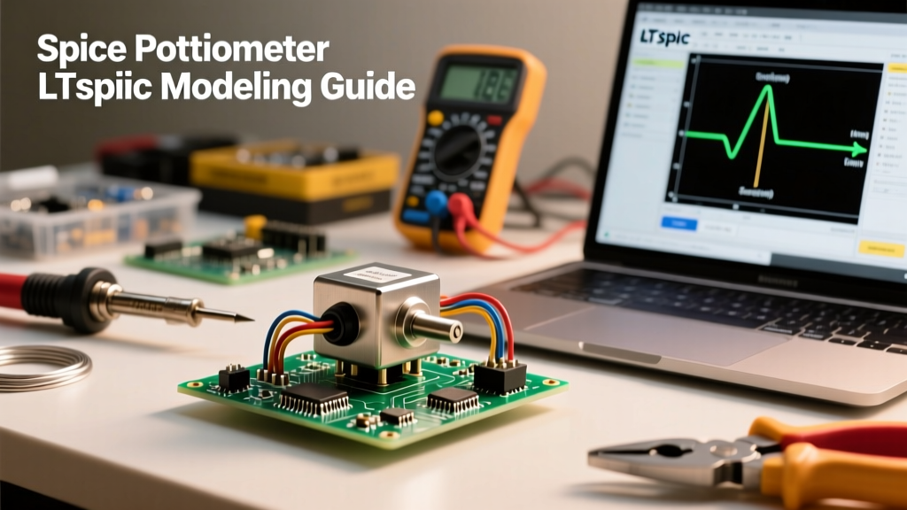

When electronics enthusiasts unbox their first physical beginner component kit, they are usually greeted by a colorful assortment of LEDs, fixed resistors, and a few rotary potentiometers. These physical variable resistors are foundational for learning voltage division, analog sensor calibration, and basic audio volume control. However, as your circuit designs grow in complexity, relying solely on physical breadboarding becomes inefficient. You must transition to virtual prototyping using circuit simulation software. This is where understanding and implementing a spice potentiometer model becomes an essential skill for any aspiring hardware engineer.
Bridging Physical and Virtual Beginner Component Kits
Standard beginner kits from brands like Elegoo or Rexqualis typically include cheap carbon-film 10kΩ linear potentiometers. While excellent for physical breadboarding, these physical components possess parasitic traits—such as wiper resistance, temperature coefficients, and mechanical noise—that basic simulations often ignore. To design robust circuits, you must bridge the gap between your physical beginner kit and your virtual workspace. By mastering SPICE (Simulation Program with Integrated Circuit Emphasis) modeling, you can predict how your physical components will behave before you ever solder a joint or route a PCB trace.
What Exactly is a SPICE Potentiometer?
Unlike fixed resistors, capacitors, or transistors, a native three-terminal variable resistor symbol does not universally exist in the base libraries of most SPICE engines, including the industry-standard LTspice by Analog Devices. A 'spice potentiometer' is not a single drag-and-drop part; rather, it is a behavioral model or a subcircuit constructed from primitive components to emulate the voltage-dividing action of a physical wiper moving across a resistive track.
For beginners transitioning from physical kits to simulation, this distinction is critical. If you attempt to sweep a resistance value in a transient analysis without a proper wiper model, your simulation will likely fail to converge or yield physically impossible results, such as infinite current spikes when the wiper approaches the ground rail.
The Two-Resistor Wiper Trick
The most straightforward way to create a spice potentiometer for basic DC operating point analysis is to use two fixed resistors in series. If you are simulating a 10kΩ potentiometer from your beginner kit set to the 60% mark, you simply place a 6kΩ resistor between the input and the wiper node, and a 4kΩ resistor between the wiper node and ground. While this works for static snapshots, it is useless for dynamic sweeping or transient analysis where you want to visualize the output voltage changing as a user physically turns the knob.
Building a Dynamic Behavioral Model in LTspice
To truly simulate a potentiometer in motion, we use behavioral resistors. In LTspice, you can define a resistor's value using an arbitrary equation. By introducing a global parameter—let us call it x, representing the wiper position from 0 to 1—we can create a dynamic spice potentiometer.
- Define the Parameter: Add a SPICE directive
.param x=0.5to set the initial wiper position. - Top Resistor (R1): Place a resistor between your input voltage and the wiper output. Right-click the resistance value and enter
{R_total * (1 - x)}. - Bottom Resistor (R2): Place a resistor between the wiper output and ground. Set its value to
{R_total * x}. - Sweep the Wiper: Use a
.step param x 0 1 0.01directive to simulate the physical rotation of the knob from 0% to 100%.
This behavioral approach perfectly mimics the linear taper (B-taper) potentiometers found in almost every entry-level electronics kit. For a deeper dive into how physical potentiometers function as voltage dividers, the SparkFun Potentiometer Basics tutorial provides an excellent foundational overview of the hardware side.
Physical vs. Simulated: Component Kit Comparison
To design effectively, you must map the physical specifications of your beginner kit components to their SPICE equivalents. Below is a comparison chart detailing how physical traits translate into simulation parameters.
| Parameter | Physical Beginner Kit Component (e.g., Carbon Film 10kΩ) | SPICE Model Equivalent | Real-World Deviation & Troubleshooting |
|---|---|---|---|
| Total Resistance | 10kΩ (±20% tolerance) | .param R_total=10k |
Physical kits have wide tolerances. Always simulate worst-case scenarios using .step for R_total at 8k and 12k. |
| Taper (Track) | Linear (B-Taper) | R = R_total * x |
Audio kits may include Logarithmic (A-Taper). Requires complex exponential SPICE equations to model accurately. |
| Wiper Resistance | 0.1Ω to 5Ω (Metal-to-carbon contact) | Fixed resistor in series with wiper node | Ignoring this causes simulated op-amp circuits to show impossible output swings near the rails. |
| Parasitic Capacitance | ~0.5pF to 2pF between terminals | Capacitors placed in parallel with R1 and R2 | Critical for high-frequency RF or audio circuits; negligible for basic DC LED dimming kits. |
The Wiper Resistance Trap: An E-E-A-T Troubleshooting Insight
One of the most common pitfalls for beginners moving from physical breadboards to SPICE simulation is the 'ideal wiper' assumption. In a purely mathematical spice potentiometer model, the wiper node has zero impedance. If you connect this ideal wiper directly to the inverting input of an op-amp or use it to pull a microcontroller GPIO pin low, the simulation will show flawless, rail-to-rail performance.
Expert Troubleshooting Tip: In reality, the physical wiper in a standard beginner kit potentiometer exhibits a contact resistance that fluctuates between 0.5Ω and 5Ω as it moves across the carbon track. If your circuit relies on the wiper pulling a node completely to 0V, this hidden resistance will create a voltage offset. Always add a
R_wiper = 2Ωfixed resistor in series with your behavioral wiper node in SPICE to catch these edge-case failures before manufacturing your PCB.
Furthermore, as physical potentiometers age or accumulate dust, this wiper resistance spikes, causing the infamous 'scratchy' sound in audio amplifiers or jittery readings in Arduino analog inputs. You can simulate this mechanical noise in SPICE by injecting a low-amplitude AC voltage source or a random behavioral noise function in series with the wiper node, allowing you to test your software's digital filtering algorithms before deploying code to your microcontroller.
Modeling Non-Linear Tapers (Audio and Anti-Log)
While beginner kits almost exclusively ship with linear (B-taper) potentiometers, advanced prototyping often requires audio taper (A-taper) or anti-log (C-taper) components. An audio taper potentiometer follows a roughly logarithmic curve, meaning the resistance changes slowly at one end of the rotation and rapidly at the other, matching the human ear's perception of loudness.
To model a logarithmic spice potentiometer, simple linear multiplication (x) is insufficient. You must implement a piecewise linear (PWL) lookup table or an exponential mathematical function within the behavioral resistor value field. For example, approximating a standard 10kΩ audio taper can be achieved using the table() function in LTspice, mapping the physical rotation angle to specific resistance breakpoints derived directly from the manufacturer's datasheet.
Translating Simulation Back to the Breadboard
The ultimate goal of mastering the spice potentiometer is to create a seamless feedback loop between virtual simulation and physical prototyping. When your SPICE model accounts for total resistance tolerance, wiper parasitics, and taper non-linearities, the transient analysis graphs on your monitor will perfectly mirror the oscilloscope traces you capture from your physical beginner kit on the workbench.
By treating your simulation environment not just as a schematic drawer, but as a highly accurate digital twin of your physical component kit, you eliminate costly PCB respins and reduce debugging time. Whether you are designing a simple voltage divider for an analog sensor or a complex feedback network for a switching power supply, accurate behavioral modeling of variable resistors is the hallmark of a mature electronics designer.