The KVL and KCL formula set forms the bedrock of all lumped-element circuit analysis. Derived from the fundamental conservation laws of physics, Kirchhoff's Voltage Law (KVL) and Kirchhoff's Current Law (KCL) allow you to predict voltage drops and branch currents in any electrical network. Whether you are sizing a current-limiting resistor for an LED or debugging a complex multi-rail PCB, these two equations are your primary diagnostic tools.
At their core, the formulas state that the directed sum of voltages around any closed loop is zero, and the directed sum of currents entering any node is zero. Below, we break down the exact mathematical definitions, the physical assumptions that make them work, and step-by-step worked examples with strict unit tracking.
The Core KVL and KCL Formula Definitions
To apply these laws correctly, you must first understand the formal summation notation. The standard mathematical representations are:
- KVL: ΣV = 0 (or Σk=1n Vk = 0)
- KCL: ΣI = 0 (or Σk=1n Ik = 0)
Symbol Definition Table
| Symbol | Definition | Standard Unit |
|---|---|---|
| Σ | Summation operator (algebraic sum of all elements in the set) | Dimensionless |
| Vk | Voltage drop or rise across the k-th element in a closed loop | Volts (V) |
| Ik | Current flowing into or out of the k-th branch connected to a node | Amperes (A) |
| k | Index variable representing a specific component or branch | Dimensionless |
| n | Total number of elements in the loop or branches at the node | Dimensionless |
Rearranged Forms for Practical Problem Solving
In practice, you rarely leave the formula as a simple summation equal to zero. You rearrange it to solve for an unknown variable. Here are the most useful algebraic rearrangements:
- KVL (Solving for an unknown voltage drop): Vunknown = Vsource - ΣVknown_drops
- KVL (Solving for an unknown source): Vsource = ΣVknown_drops
- KCL (Solving for an unknown incoming current): Iin_unknown = ΣIout - ΣIin_known
- KCL (Solving for an unknown outgoing current): Iout_unknown = ΣIin - ΣIout_known
Assumptions, Limits, and Unit Traps
The KVL and KCL formula set is not a universal law of the universe; it is an approximation that relies on the lumped element model. According to MIT OpenCourseWare's Circuits and Electronics curriculum, this model assumes that the physical dimensions of your circuit are significantly smaller than the wavelength of the electrical signals passing through it.
When the Formula Applies (and When It Breaks)
For standard DC circuits or 60Hz AC mains power, the wavelength is thousands of kilometers. Your PCB or home wiring is mere meters long, so the lumped element assumption holds perfectly. However, if you are designing an RF layout for an ESP32 transmitting at 2.4 GHz, the wavelength is roughly 12.5 cm. If your PCB traces approach 1.25 cm (1/10th of the wavelength), the traces act as transmission lines. Parasitic capacitance and inductance dominate, energy radiates into space, and the standard KVL and KCL formula calculations will yield incorrect results. You must use Maxwell's equations and S-parameters instead.
Unit Mistakes That Break Your Math
The most common reason hobbyists and students get wildly incorrect answers is failing to normalize units before summing. The summation operator requires all terms to share the exact same base unit.
If you have a 50 mA branch and a 0.1 A branch meeting at a node, you cannot write 50 + 0.1 = 50.1 A. You must convert both to Amperes (0.050 A + 0.1 A = 0.15 A) or both to milliamperes (50 mA + 100 mA = 150 mA). Always write the units next to your numbers during intermediate steps.
What a Realistic Answer Magnitude Looks Like
Developing an intuition for realistic magnitudes acts as a sanity check. In low-voltage hobby electronics (3.3V to 24V systems), branch currents typically range from 1 mA to 2 A. If your KCL calculation tells you a logic gate is sourcing 450 A, you have missed a decimal point or forgotten to convert milliohms to ohms. As noted by Georgia State University's HyperPhysics, checking the order of magnitude against physical reality is a critical step in circuit verification.
Worked Example 1: KVL in a Series DC Loop
Scenario: You are designing a simple indicator circuit. You have a 12V DC power supply, a standard red LED with a forward voltage (Vf) of 2.1V, and you need to limit the current to exactly 20 mA (0.020 A) to prevent thermal runaway. Use the KVL and KCL formula principles to find the required resistance (R) and its minimum power rating.
Step 1: Define the loop and current direction.
Assume a clockwise current flow starting from the positive terminal of the 12V source.
Step 2: Write the KVL equation.
+Vsource - VLED - VR = 0
Step 3: Substitute known values with units.
+12V - 2.1V - VR = 0
9.9V - VR = 0
VR = 9.9V
Step 4: Apply Ohm's Law to find R.
R = VR / I
R = 9.9V / 0.020A
R = 495 Ω
Step 5: Select a standard component and verify power.
The closest standard E24 series resistor is 510 Ω. Let's verify the power dissipation to ensure the resistor doesn't burn up.
P = I² × R
P = (0.020A)² × 510Ω
P = 0.0004 × 510 = 0.204 W
Since 0.204 W is close to the limit of a standard 1/4W (0.25W) resistor, a prudent engineer will step up to a 1/2W (0.5W) resistor for thermal reliability.
Worked Example 2: KCL at a Multi-Branch Node
Scenario: You are debugging a custom 5V sensor board. The main 5V rail enters a distribution node. From this node, three branches emerge: one feeds an ESP32-WROOM-32 module (drawing an average of 80 mA), one feeds a logic-level MOSFET gate driver (drawing 15 mA), and the third feeds an unknown analog sensor. Your multimeter measures the total current entering the node from the main supply as 125 mA. Find the current drawn by the analog sensor.
Step 1: Define the node and assign signs.
Let current entering the node be positive (+), and current leaving the node be negative (-).
Step 2: Write the KCL equation.
ΣI = 0
Iin - IESP32 - Idriver - Isensor = 0
Step 3: Normalize units and substitute.
All values are already in mA, so we can proceed safely.
125 mA - 80 mA - 15 mA - Isensor = 0
Step 4: Solve for the unknown.
125 mA - 95 mA - Isensor = 0
30 mA - Isensor = 0
Isensor = 30 mA
Step 5: Practical verification.
The sensor draws 30 mA. If this sensor is an I2C temperature probe like the TMP117, a 30 mA draw indicates a fault, as it should only draw microamps. The KCL math is correct, but the physical circuit likely has a short or a failed decoupling capacitor on the sensor branch.
Frequently Asked Questions
Does the KVL and KCL formula work for AC circuits?
Yes, but you must use complex numbers (phasors) instead of simple scalars. In AC analysis, voltages and currents have both magnitude and phase. The KVL and KCL formula still holds true, meaning the vector sum of all complex voltages around a loop is zero, and the vector sum of all complex currents at a node is zero. You cannot simply add the RMS magnitudes together; you must account for the phase angle shift introduced by capacitors and inductors.
Why do my KVL and KCL formula calculations fail on high-frequency RF PCBs?
At high frequencies, the physical size of the circuit traces becomes a significant fraction of the signal's wavelength. The lumped element model breaks down because voltage and current are no longer uniform across a component at a single instant in time. Energy is stored in the parasitic capacitance between traces and parasitic inductance of the copper itself, and some energy radiates away as electromagnetic waves. In these scenarios, you must abandon basic Kirchhoff laws and use transmission line theory and S-parameters.
How do I handle dependent sources when using the KVL and KCL formula?
Dependent sources (like a voltage-controlled voltage source in an op-amp model) are treated exactly like independent sources when writing your initial KVL and KCL equations. However, they introduce an extra variable. To solve the system, you must write an additional 'controlling equation' that defines the dependent source's value in terms of another voltage or current in the circuit. You then use substitution or matrix algebra (like Cramer's rule) to solve the expanded system of linear equations.